
Example: Score-Based Generative Model for 2D Swiss Roll Dataset#
This example is based on Yang Song’s Google Colab Tutorial. However we changed the data to be a 2D Swiss Roll dataset like in the ScoreDiffusionModel repository.
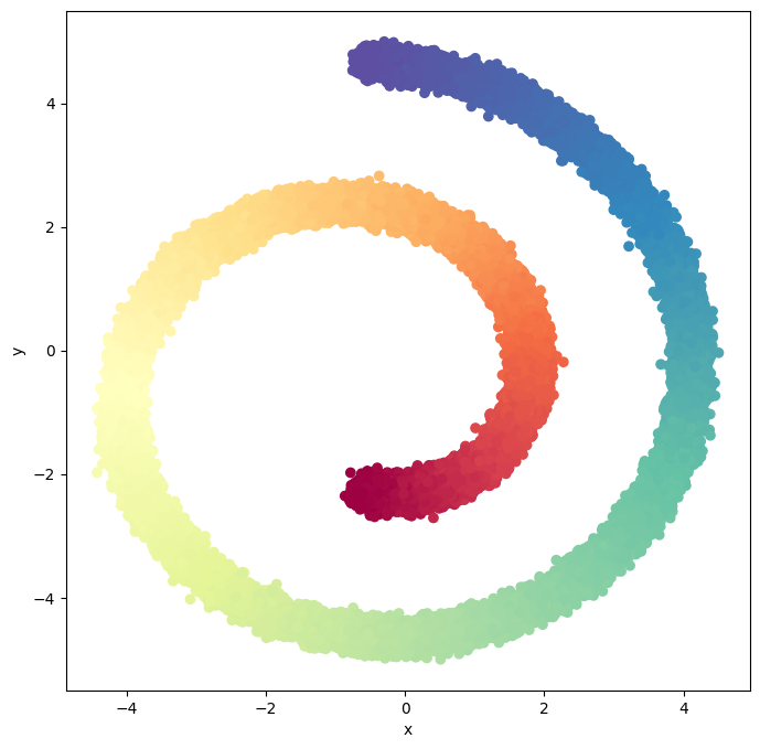
Generate Swiss Roll Dataset#
First, we generate a noise disturbed 2D Swiss Roll dataset with 100000 samples. We will use this dataset to train our score-based generative model.
from sklearn.datasets import make_swiss_roll
import numpy as np
import torch
import torch.nn as nn
import matplotlib.pyplot as plt
import matplotlib.animation as animation
from IPython.display import HTML
from IPython.display import clear_output
import functools
from torch.optim import Adam
from torch.utils.data import DataLoader
from tqdm.notebook import trange
# Set the device
device = 'mps' # 'cuda' or 'cpu'
def generate_swiss_roll_dataset(n_samples=1000, noise=0.0, random_state=None):
"""
Function to generate Swiss Roll dataset.
Parameters:
n_samples (int): The total number of points equally divided among classes.
noise (float): Standard deviation of Gaussian noise added to the data.
random_state (int): Determines random number generation for dataset creation.
Returns:
X (torch.Tensor): The generated samples.
t (torch.Tensor): The univariate position of the sample according to the main dimension of the points in the Swiss Roll.
"""
X, t = make_swiss_roll(n_samples, noise=noise, random_state=random_state)
X = X[:, [0, 2]]
# Scale and normalize to [-1,1]
X = (X - np.min(X)) / (np.max(X) - np.min(X))
X = 10 * X - 5
# Convert to PyTorch tensors
X = torch.from_numpy(X).float()
t = torch.from_numpy(t).float()
return X, t
# Generate Swiss Roll dataset
X, t = generate_swiss_roll_dataset(n_samples=100000, noise=0.3, random_state=42)
print(f"Swiss Roll dataset: {X.shape}")
print(f"Labels: {t.shape}")
Swiss Roll dataset: torch.Size([100000, 2])
Labels: torch.Size([100000])
# function to Plot 2d Swiss Roll dataset
def plot_2d_swiss_roll(X, t=None, title="Swiss Roll data"):
if t is None:
t = np.zeros(X.shape[0])
fig = plt.figure(figsize=(8, 8))
ax = fig.add_subplot(111)
ax.scatter(X[:, 0], X[:, 1], c=t, cmap=plt.cm.Spectral)
ax.set_xlabel("x")
ax.set_ylabel("y")
plt.show()
plot_2d_swiss_roll(X, t, title="Swiss Roll dataset")
Implmeneting Score-Based Generative Model#
Encoding the time information#
We can incorporate the time information via Gaussian random features. Specifically, we first sample \(\omega \sim \mathcal{N}(\mathbf{0}, s^2\mathbf{I})\) which is subsequently fixed for the model (i.e., not learnable). For a time step \(t\), the corresponding Gaussian random feature is defined as
where \([\vec{a} ; \vec{b}]\) denotes the concatenation of vector \(\vec{a}\) and \(\vec{b}\). This Gaussian random feature can be used as an encoding for time step \(t\) so that the score network can condition on \(t\) by incorporating this encoding. We will see this further in the code.
class GaussianFourierProjection(nn.Module):
"""Gaussian random features for encoding time steps."""
# [\sin(2\pi \omega t) ; \cos(2\pi \omega t)]
def __init__(self, embed_dim, scale=30.):
super().__init__()
# Randomly sample weights during initialization. These weights are fixed
# during optimization and are not trainable.
self.W = nn.Parameter(torch.randn(embed_dim // 2) * scale, requires_grad=False)
def forward(self, x):
x_proj = x[:, None] * self.W[None, :] * 2 * np.pi
return torch.cat([torch.sin(x_proj), torch.cos(x_proj)], dim=-1)
Define the Score-Based Model#
class ScoreNet(nn.Module):
def __init__(self, marginal_prob_std, input_dim=2, hidden_dim=512, output_dim=2, embed_dim=256):
super().__init__()
# Gaussian random feature embedding layer for time
self.embed = nn.Sequential(GaussianFourierProjection(embed_dim=embed_dim),
nn.Linear(embed_dim, embed_dim),
nn.GELU()
)
self.linear_model1 = nn.Sequential(
nn.Linear(input_dim, embed_dim),
nn.Dropout(0.2),
nn.GELU()
)
self.linear_model2 = nn.Sequential(
nn.Linear(embed_dim, hidden_dim),
nn.Dropout(0.2),
nn.GELU(),
nn.Linear(hidden_dim, hidden_dim),
nn.Dropout(0.2),
nn.GELU(),
nn.Linear(hidden_dim, input_dim),
)
self.marginal_prob_std = marginal_prob_std
def forward(self, x, t):
h = self.linear_model2(self.linear_model1(x) + self.embed(t))/ self.marginal_prob_std(t)[:, None]
return h
Training with Weighted Sum of Denoising Score Matching Objectives#
As discussed in the previous section we want to train our score-based model on a denoising score matching objective. Hence, to train our model, we need to specify an SDE that perturbs the data distribution \(p_0\) to a prior distribution \(p_T\). We choose the following SDE
Note that in this SDE our drift term is zero and our diffusion term is based on the Wiener process \(d{w}\).
In this case,
and we can choose the weighting function \(\lambda(t) = \frac{1}{2 \log \sigma}(\sigma^{2t} - 1)\).
When \(\sigma\) is large, the prior distribution, \(p_{t=1}\) is
which is approximately independent of the data distribution and is easy to sample from.
Intuitively, this SDE captures a continuum of Gaussian perturbations with variance function \(\frac{1}{2 \log \sigma}(\sigma^{2t} - 1)\). This continuum of perturbations allows us to gradually transfer samples from a data distribution \(p_0\) to a simple Gaussian distribution \(p_1\).
def marginal_prob_std(t, sigma):
"""Compute the mean and standard deviation of $p_{0t}(x(t) | x(0))$.
Args:
t: A vector of time steps.
sigma: The $\sigma$ in our SDE.
Returns:
The standard deviation.
"""
t = torch.tensor(t, device=device)
return torch.sqrt((sigma**(2 * t) - 1.) / 2. / np.log(sigma))
def diffusion_coeff(t, sigma):
"""Compute the diffusion coefficient of our SDE.
Args:
t: A vector of time steps.
sigma: The $\sigma$ in our SDE.
Returns:
The vector of diffusion coefficients.
"""
return torch.tensor(sigma**t, device=device)
sigma = 25.0
marginal_prob_std_fn = functools.partial(marginal_prob_std, sigma=sigma)
diffusion_coeff_fn = functools.partial(diffusion_coeff, sigma=sigma)
Define the Denoising Score Matching Loss Function#
We can train a time-dependent score-based model \(s_\theta(\mathbf{x}, t)\) to approximate \(\nabla_\mathbf{x} \log p_t(\mathbf{x})\), using the following weighted sum of denoising score matching objectives.
where \(\mathcal{U}(0,T)\) is a uniform distribution over \([0, T]\) and \(\lambda(t) \in \mathbb{R}_{>0}\) denotes a positive weighting function. In the objective, the expectation over \(\mathbf{x}(0)\) can be estimated with empirical means over data samples from \(p_0\). The expectation over \(\epsilon\) can be estimated by sampling from \(\mathcal{N}(0, \mathbf{I})\) and is used to transform the samples from \(x_0\) to \(x_t\).
Note that we do not have to consider the weight function \(\lambda(t)\) in the implementation of the loss function, since we chose the variance of the noise \(\epsilon\) and \(\lambda(t)\) to be the same. Hence, they cancel out in the loss function.
def loss_fn(model, x, marginal_prob_std, eps=1e-5):
random_t = torch.rand(x.shape[0], device=x.device) * (1. - eps) + eps
z = torch.randn_like(x)
std = marginal_prob_std(random_t)
perturbed_x = x + z * std[:, None]
score = model(perturbed_x, random_t)
loss = torch.mean(torch.sum((score * std[:, None] + z)**2, dim=1))
return loss
Initialize the network#
# network parameter
input_dim = 2 # x, y coordinates
hidden_dim = 512 # hidden dimension
output_dim = 2 # Score for each coordinate
embed_dim = 256 # Dimension of the Gaussian random feature embedding
# marginal_prob_std, input_dim=2, hidden_dim=32, output_dim=2, embed_dim=16
score_model = ScoreNet(marginal_prob_std_fn, input_dim, hidden_dim, output_dim, embed_dim)
score_model = score_model.to(device)
Set the Training parameter and load the data#
# set to True if you have a pre-trained model
load_model = True
if load_model:
ckpt = torch.load('score_ckpt.pth', map_location=device)
score_model.load_state_dict(ckpt)
# Training parameters
batch_size = 8192 # size of a mini-batch 8192
n_epochs = 0 # number of training epochs 40 is good
lr = 1e-3 # learning rate 1e-3
# Loss function parameters
eps = 1e-3 # epsilon for numerical stability 1e-5
# Prepare the data loader
X_tensor = torch.tensor(X, dtype=torch.float32, device=device)
t_tensor = torch.tensor(t, dtype=torch.float32, device=device)
data_loader = DataLoader(
list(zip(X_tensor, t_tensor)),
batch_size=batch_size,
shuffle=True,
num_workers=0
)
/var/folders/59/r58bsq3j6j9f_t7d4z2fbww40000gn/T/ipykernel_24913/3234266540.py:15: UserWarning: To copy construct from a tensor, it is recommended to use sourceTensor.clone().detach() or sourceTensor.clone().detach().requires_grad_(True), rather than torch.tensor(sourceTensor).
X_tensor = torch.tensor(X, dtype=torch.float32, device=device)
/var/folders/59/r58bsq3j6j9f_t7d4z2fbww40000gn/T/ipykernel_24913/3234266540.py:16: UserWarning: To copy construct from a tensor, it is recommended to use sourceTensor.clone().detach() or sourceTensor.clone().detach().requires_grad_(True), rather than torch.tensor(sourceTensor).
t_tensor = torch.tensor(t, dtype=torch.float32, device=device)
Training the score model#
optimizer = Adam(score_model.parameters(), lr=lr)
tqdm_epoch = trange(n_epochs)
for epoch in tqdm_epoch:
avg_loss = 0.
num_items = 0
for x, y in data_loader:
# x = torch.tensor(x, dtype=torch.float32).to(device)
loss = loss_fn(score_model, x, marginal_prob_std_fn, eps=eps)
optimizer.zero_grad()
loss.backward()
optimizer.step()
avg_loss += loss.item() * x.shape[0]
num_items += x.shape[0]
# Print the averaged training loss so far.
tqdm_epoch.set_description('Average Loss: {:5f}'.format(avg_loss / num_items))
# Update the checkpoint after each epoch of training.
torch.save(score_model.state_dict(), 'score_ckpt.pth')
Defining the sampling function - Numerical sampling based on score SDE#
Recall that for any SDE of the form
the reverse-time SDE is given by
where, \(p_t(x_t)\) is the probability density function of the data distribution at time \(t\).
Since we have chosen the forward SDE (without a drift term) to be
The reverse-time SDE is given by
To sample from our time-dependent score-based model \(s_\theta({x}, t)\), we first draw a sample from the prior distribution
and then solve the reverse-time SDE with numerical methods.
In particular, using our time-dependent score-based model, the reverse-time SDE can be approximated by
Next, one can use numerical methods to solve for the reverse-time SDE, such as the Euler-Maruyama approach. It is based on a simple discretization to the SDE, replacing \(dt\) with \(\Delta t\) and \(d {w}\) with \({z} \sim \mathcal{N}({0}, g^2(t) \Delta t {I})\). When applied to our reverse-time SDE, we can obtain the following iteration rule
where \({z}_t \sim \mathcal{N}({0}, {I})\).
def Euler_Maruyama_sampler(score_model,
marginal_prob_std,
diffusion_coeff,
batch_size=64,
num_steps=100,
device='mps',
eps=1e-5):
t = torch.ones(batch_size, device=device)
init_x = torch.randn(batch_size, input_dim, device=device) * marginal_prob_std(t)[:, None]
time_steps = torch.linspace(1., eps, num_steps, device=device)
step_size = time_steps[0] - time_steps[1]
x = init_x
with torch.no_grad():
for time_step in time_steps:
batch_time_step = torch.ones(batch_size, device=device) * time_step
g = diffusion_coeff(batch_time_step)
x_mean = x + (g**2)[:, None] * score_model(x, batch_time_step) * step_size
x = x_mean + torch.sqrt(g**2 * step_size)[:, None] * torch.randn_like(x)
# Do not include any noise in the last sampling step.
return x_mean
Better Solver - SDE based predictor corrector sampling#
Aside from generic numerical SDE solvers, we can leverage special properties of our reverse-time SDE for better solutions. Since we have an estimate of the score of \(p_t({x}(t))\) via the score-based model, i.e., \(s_\theta({x}, t) \approx \nabla_{{x}(t)} \log p_t({x}(t))\), we can leverage score-based MCMC approaches, such as Langevin MCMC, to correct the solution obtained by numerical SDE solvers.
Score-based MCMC approaches can produce samples from a distribution \(p({x})\) once its score \(\nabla_{x} \log p({x})\) is known. For example, Langevin MCMC operates by running the following iteration rule for \(i=1,2,\cdots, N\):
where \({z}_i \sim \mathcal{N}({0}, {I})\), \(\epsilon > 0\) is the step size, and \({x}_1\) is initialized from any prior distribution \(\pi({x}_1)\). When \(N\to\infty\) and \(\epsilon \to 0\), the final value \({x}_{N+1}\) becomes a sample from \(p({x})\) under some regularity conditions. Therefore, given \(s_\theta({x}, t) \approx \nabla_{x} \log p_t({x})\), we can get an approximate sample from \(p_t({x})\) by running several steps of Langevin MCMC, replacing \(\nabla_{x} \log p_t({x})\) with \(s_\theta({x}, t)\) in the iteration rule.
Predictor-Corrector samplers combine both numerical solvers for the reverse-time SDE and the Langevin MCMC approach. In particular, we first apply one step of numerical SDE solver to obtain \({x}_{t-\Delta t}\) from \({x}_t\), which is called the “predictor” step. Next, we apply several steps of Langevin MCMC to refine \({x}_t\), such that \({x}_t\) becomes a more accurate sample from \(p_{t-\Delta t}({x})\). This is the “corrector” step as the MCMC helps reduce the error of the numerical SDE solver.
def pc_sampler(score_model,
marginal_prob_std,
diffusion_coeff,
batch_size=64,
num_steps=400,
snr=0.16,
device='mps',
eps=1e-5):
t = torch.ones(batch_size, device=device)
init_x = torch.randn(batch_size, input_dim, device=device) * marginal_prob_std(t)[:, None]
time_steps = np.linspace(1., eps, num_steps)
step_size = time_steps[0] - time_steps[1]
x = init_x
samples = []
with torch.no_grad():
for time_step in time_steps:
batch_time_step = torch.ones(batch_size, device=device) * time_step
# Corrector step (Langevin MCMC)
grad = score_model(x, batch_time_step)
grad_norm = torch.norm(grad, dim=-1).mean()
noise_norm = np.sqrt(np.prod(x.shape[1:]))
langevin_step_size = 2 * (snr * noise_norm / grad_norm)**2
x = x + langevin_step_size * grad + torch.sqrt(2 * langevin_step_size) * torch.randn_like(x)
# Predictor step (Euler-Maruyama)
g = diffusion_coeff(batch_time_step)
x_mean = x + (g**2)[:, None] * score_model(x, batch_time_step) * step_size
x = x_mean + torch.sqrt(g**2 * step_size)[:, None] * torch.randn_like(x)
samples.append(x_mean.cpu().clone().numpy())
samples = np.stack(samples, axis=1)
time_series_samples = np.swapaxes(samples, 0, 1)
# The last step does not include any noise
return x_mean, time_series_samples
Testing the score model using predictor corrector sampling#
num_steps = 400
signal_to_noise_ratio = 0.015
eps = 1e-3
num_samples = 2000
# Test the prdictor corrector sample function
last_sample, sample_time_series = pc_sampler(score_model, marginal_prob_std_fn, diffusion_coeff_fn, num_steps=num_steps, batch_size=num_samples, device=device, snr=signal_to_noise_ratio, eps=eps)
/var/folders/59/r58bsq3j6j9f_t7d4z2fbww40000gn/T/ipykernel_24913/74995779.py:11: UserWarning: To copy construct from a tensor, it is recommended to use sourceTensor.clone().detach() or sourceTensor.clone().detach().requires_grad_(True), rather than torch.tensor(sourceTensor).
t = torch.tensor(t, device=device)
/var/folders/59/r58bsq3j6j9f_t7d4z2fbww40000gn/T/ipykernel_24913/74995779.py:24: UserWarning: To copy construct from a tensor, it is recommended to use sourceTensor.clone().detach() or sourceTensor.clone().detach().requires_grad_(True), rather than torch.tensor(sourceTensor).
return torch.tensor(sigma**t, device=device)
scatter_range = [-7, 7]
# only take the last xx% of the samples for visualization
# num_step = sample_time_series.shape[0]
# sample_time_series = sample_time_series[int(num_step*0.1):, :, :]
sample = torch.tensor(sample_time_series, dtype=torch.float32, device=device)
def update_plot(i, data, scat):
scat.set_offsets(data[i].detach().cpu().numpy())
return scat
numframes = len(sample)
scatter_point = sample[0].detach().cpu().numpy()
scatter_x, scatter_y = scatter_point[:,0], scatter_point[:,1]
fig = plt.figure(figsize=(6, 6))
plt.xlim(scatter_range)
plt.ylim(scatter_range)
scat = plt.scatter(scatter_x, scatter_y, s=1)
plt.show()
clear_output()
ani = animation.FuncAnimation(fig, update_plot, frames=range(numframes), fargs=(sample, scat), interval=150)
writergif = animation.PillowWriter(fps=50)
ani.save('score_swiss.gif', writer=writergif)
HTML(ani.to_jshtml())