
Illustration of Diffusion Process#
I want to note that this notebook has been lightly modified from its original form, sourced from the DiffusionFastForward repository: mikonvergence/DiffusionFastForward
In this notebook, the intricacies of a denosing diffusion framework are illustrated with the aid of simple snippets.
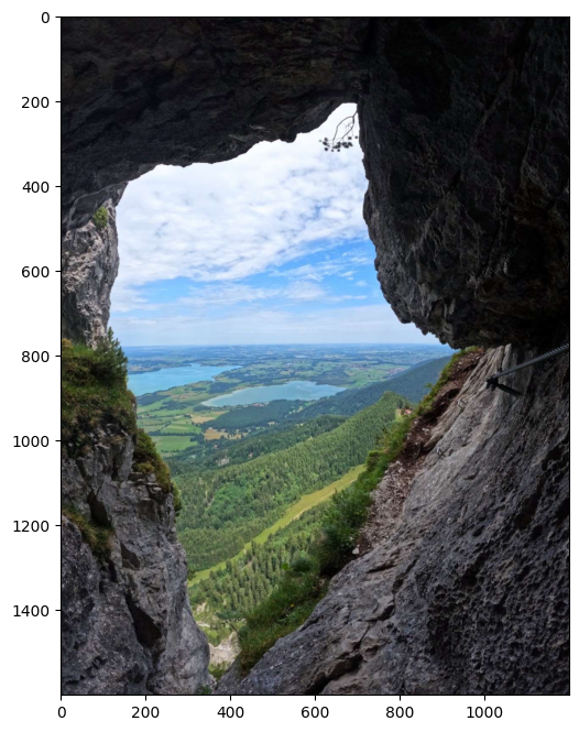
First, let’s import an image to use for the examples.
import torch
import torch.nn.functional as F
import numpy as np
import matplotlib as mpl
import matplotlib.pyplot as plt
import imageio

mpl.rcParams['figure.figsize'] = (12, 8)

# img = torch.FloatTensor(imageio.imread('imgs/hills_2.png')/255)
img = torch.FloatTensor(imageio.imread('imgs/Klettersteig.jpg')/255)
plt.imshow(img)
/var/folders/59/r58bsq3j6j9f_t7d4z2fbww40000gn/T/ipykernel_24876/3026492335.py:11: DeprecationWarning: Starting with ImageIO v3 the behavior of this function will switch to that of iio.v3.imread. To keep the current behavior (and make this warning disappear) use `import imageio.v2 as imageio` or call `imageio.v2.imread` directly.
  img = torch.FloatTensor(imageio.imread('imgs/Klettersteig.jpg')/255)
<matplotlib.image.AxesImage at 0x17d764d60>

Data Preprocessing#
The majority of the diffusion models assume that the images are scaled to the [-1,+1] range (which tends to simplify many equations). This tutorial will follow the same approach, so we need to define input and output transformation functions input_T() and output_T().
Also, let’s define our own show() wrapper function that displays the image with automatic output transformation!
def input_T(input):
    # [0,1] -> [-1,+1]
    return 2*input-1

def output_T(input):
    # [-1,+1] -> [0,1]
    return (input+1)/2

def show(input):
    plt.imshow(output_T(input).clip(0,1))

img_=input_T(img)
show(img_)
Defining a schedule#
The diffusion process is built based on a variance schedule, which determines the levels of added noise at each step of the process. To that end, our schedule is defined below, with the following quantities:
betas:\(\beta_t \in [0, 1]\)alphas: \(\alpha_t=1-\beta_t\)alphas_sqrt: \(\sqrt{\alpha_t}\)alphas_prod: \(\bar{\alpha}_t=\prod_{i=0}^{t}\alpha_i\)alphas_prod_sqrt: \(\sqrt{\bar{\alpha}_t}\)
num_timesteps=1000
betas=torch.linspace(1e-4,2e-2,num_timesteps)   # from 0.0001 to 0.02 in 1000 steps

alphas=1-betas                                  # from 0.9999 to 0.98 in 1000 steps
alphas_sqrt=alphas.sqrt()
alphas_cumprod=torch.cumprod(alphas,0)
alphas_cumprod_sqrt=alphas_cumprod.sqrt()
Forward Process#
The forward process \(q\) determines how subsequent steps in the diffusion are derived (gradual distortion of the original sample \(x_0\)).
📃 First, let’s bring up the key equations describing this process…
Basic format of the forward step: $\( q(x_t|x_{t−1}) := \mathcal{N}(x_t; \sqrt{1 − \beta_t}x_{t−1}, \beta_tI) \tag{1} \)$
For a complete trajectory \(x_{0}\) to \(x_{1:T}\) We can describe it with the following product of conditional distributions: $\( q(\mathbf{x}_{1:T} \vert \mathbf{x}_0) = \prod^T_{t=1} q(\mathbf{x}_t \vert \mathbf{x}_{t-1}) \)$
For infinite steps \(T \rightarrow \infty\) the input data would be transformed into a variable from an isotropic Gaussian distribution \(x_T \sim N(0,I)\).
To step directly from \(x_0\) to \(x_t\) we can use the reparmetrization trick (with \(\bar{\alpha_t}=\prod^t_{i=1}\alpha_i\)): $\( q(x_t|x_0) = \mathcal{N}(x_t;\sqrt{\bar{\alpha_t}}x_0, (1 − \bar{\alpha_t})I) \tag{2} \)$
Forward Step#
Let’s define a function forward_step() that will allow us to use both \(q(x_t|x_{t-1})\) and forward_jump() for \(q(x_t|x_0)\)
def forward_step(t, condition_img, return_noise=False):
    """
        forward step: t-1 -> t
    """
    assert t >= 0

    mean=alphas_sqrt[t]*condition_img
    std=betas[t].sqrt()

    # sampling from N
    if not return_noise:
        return mean+std*torch.randn_like(img)
    else:
        noise=torch.randn_like(img)
        return mean+std*noise, noise

def forward_jump(t, condition_img, condition_idx=0, return_noise=False):
    """
        forward jump: 0 -> t
    """
    assert t >= 0

    mean=alphas_cumprod_sqrt[t]*condition_img
    std=(1-alphas_cumprod[t]).sqrt()

    # sampling from N
    if not return_noise:
        return mean+std*torch.randn_like(img)
    else:
        noise=torch.randn_like(img)
        return mean+std*noise, noise
N=5 # number of computed states between x_0 and x_T
M=4 # number of samples taken from each distribution
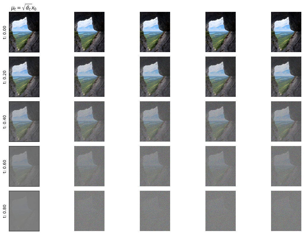
In the first example, when t==0, we want to derive a sample \(x_t\) based on the clean sample \(x_0\)!
The first column shows the mean image for a given stage of the diffusion, and the subsequent columns to the right show several samples taken from the same distribution (they are different if you look closely!).
plt.figure(figsize=(12,8))
for idx in range(N):
    t_step=int(idx*(num_timesteps/N))

    plt.subplot(N,1+M,1+(M+1)*idx)
    show(alphas_cumprod_sqrt[t_step]*img_)
    plt.title(r'$\mu_t=\sqrt{\bar{\alpha}_t}x_0$') if idx==0 else None
    plt.ylabel("t: {:.2f}".format(t_step/num_timesteps))
    plt.xticks([])
    plt.yticks([])

    for sample in range(M):
        x_t=forward_jump(t_step,img_)

        plt.subplot(N,1+M,2+(1+M)*idx+sample)
        show(x_t)
        plt.axis('off')

plt.tight_layout()
Alternatively, we can test the process of going from \(x_{t-1}\) to \(x_t\), which is a single step in the diffusion process. For that we can use the forward_step function.
Note that the mean \(\mu_t\) is now a bit different (first column) since it is conditioned on a specific sample of \(x_{t-1}\)!
plt.figure(figsize=(12,8))
for idx in range(N):
    t_step=int(idx*(num_timesteps/N))
    prev_img=forward_jump(max([0,t_step-1]),img_) # directly go to prev state

    plt.subplot(N,1+M,1+(M+1)*idx)
    show(alphas_sqrt[t_step]*prev_img)
    plt.title(r'$\mu_t=\sqrt{1-\beta_t}x_{t-1}$') if idx==0 else None
    plt.ylabel("t: {:.2f}".format(t_step/num_timesteps))
    plt.xticks([])
    plt.yticks([])

    for sample in range(M):
        plt.subplot(N,1+M,2+(1+M)*idx+sample)
        x_t=forward_step(t_step,prev_img)
        show(x_t)
        plt.axis('off')
plt.tight_layout()

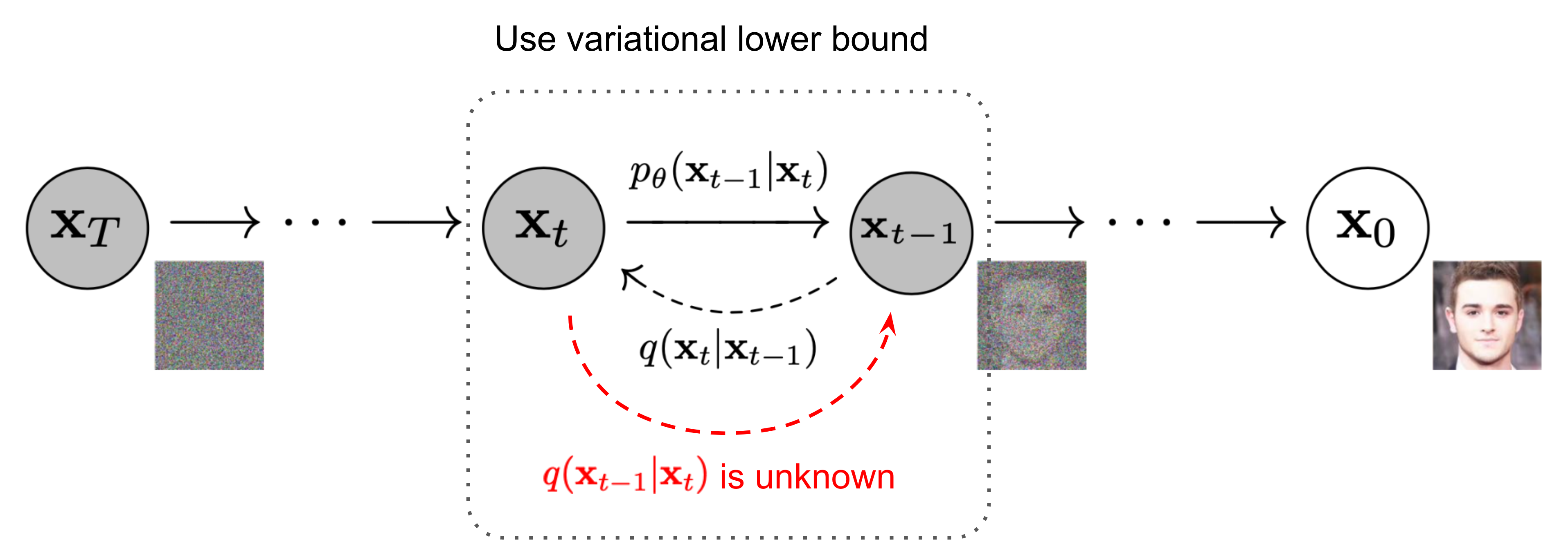
Reverse Process#
The purpose of the reverse process \(p\) is to approximate the previous step \(x_{t-1}\) in the diffusion chain based on a sample \(x_t\). In practice, this approximation \(p(x_{t-1}|x_t)\) must be done without the knowledge of \(x_0\).
A parametrizable prediction model with parameters \(\theta\) is used to estimate \(p_\theta(x_{t-1}|x_t)\).
The reverse process will also be (approximately) gaussian if the diffusion steps are small enough:
In many works, it is assumed that the variance of this distribution should not depend strongly on \(x_0\) or \(x_t\), but rather on the stage of the diffusion process \(t\). This can be observed in the true distribution \(q(x_{t-1}|x_t, x_0)\), where the variance of the distribution equals \(\tilde{\beta}_t\).
Parameterizing \(\mu_\theta\)#
There are at least 3 ways of parameterizing the mean of the reverse step distribution \(p_\theta(x_{t-1}|x_t)\):
Directly (a neural network will estimate \(\mu_\theta\)) $\(\mu_\theta = \mu_\theta(x_t,t)\)$
Via \(x_0\) (a neural network will estimate \(x_0\)) $\(\tilde{\mu}_\theta = \frac{\sqrt{\bar{\alpha}_{t-1}}\beta_t}{1-\bar{\alpha}_t}x_{0, \theta}(x_t,t) + \frac{\sqrt{\alpha_t}(1-\bar{\alpha}_{t-1})}{1-\bar{\alpha}_t}x_t \tag{4}\)$
Via noise \(\epsilon\) subtraction from \(x_t\) (a neural network will estimate \(\epsilon\)) $\(x_0=\frac{1}{\sqrt{\bar{\alpha}_t}}(x_t-\sqrt{1-\bar{\alpha}_t} \epsilon_\theta(x_t,t))\tag{5}\)$
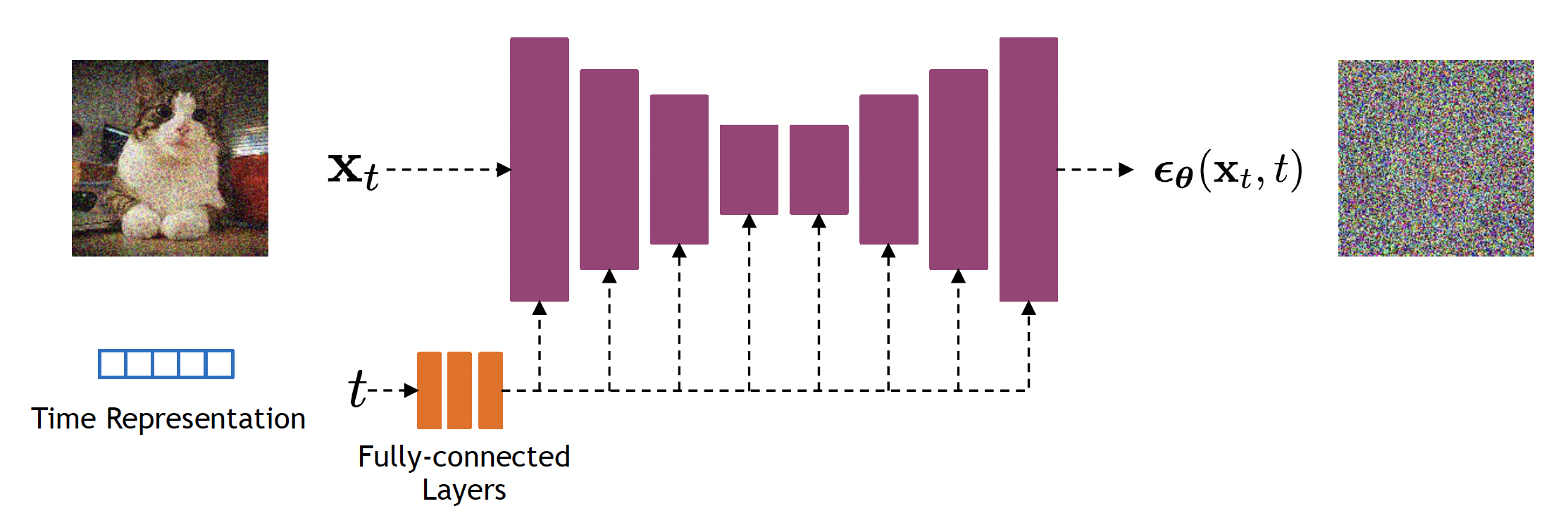
Approach 3 of approximating the normal noise \(\epsilon_\theta\) is used most widely.
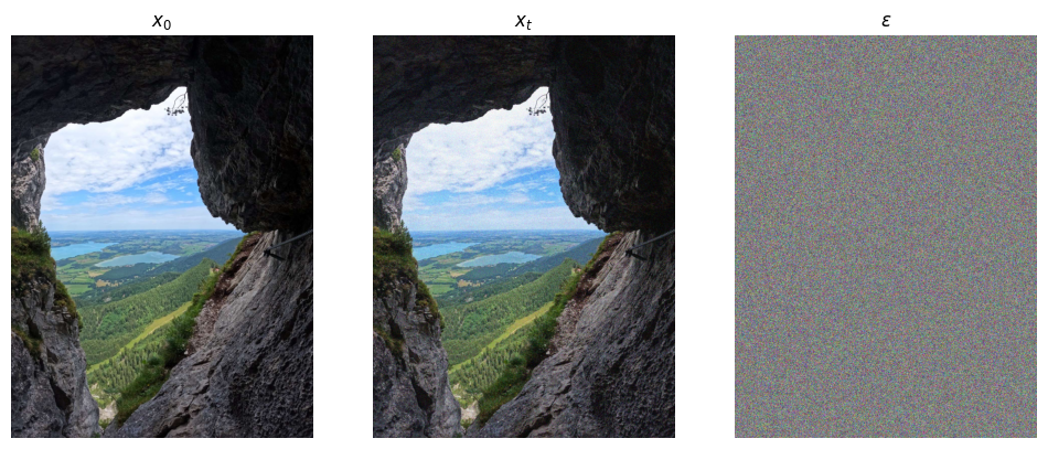
Example, estimating \(\epsilon\) using a U-Net:
Let’s look at what an example \(\epsilon\) might look like:
t_step=50

x_t,noise=forward_jump(t_step,img_,return_noise=True)

plt.subplot(1,3,1)
show(img_)
plt.title(r'$x_0$')
plt.axis('off')
plt.subplot(1,3,2)
show(x_t)
plt.title(r'$x_t$')
plt.axis('off')
plt.subplot(1,3,3)
show(noise)
plt.title(r'$\epsilon$')
plt.axis('off')
(-0.5, 1199.5, 1599.5, -0.5)
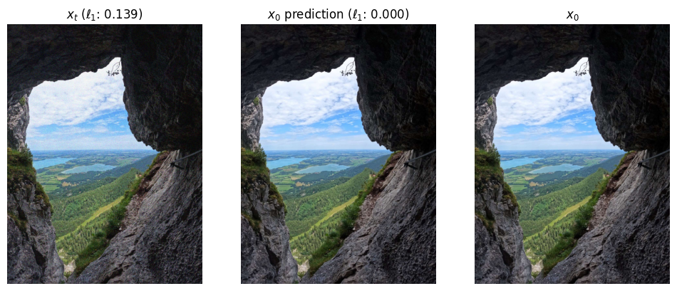
If \(\epsilon\) is predicted correctly, we can use the equation (5) to predict \(x_0\):
x_0_pred=(x_t-(1-alphas_cumprod[t_step]).sqrt()*noise)/(alphas_cumprod_sqrt[t_step])

plt.subplot(1,3,1)
show(x_t)
plt.title('$x_t$ ($\ell_1$: {:.3f})'.format(F.l1_loss(x_t,img_)))
plt.axis('off')
plt.subplot(1,3,2)
show(x_0_pred)
plt.title('$x_0$ prediction ($\ell_1$: {:.3f})'.format(F.l1_loss(x_0_pred,img_)))
plt.axis('off')
plt.subplot(1,3,3)
show(img_)
plt.title('$x_0$')
plt.axis('off')
(-0.5, 1199.5, 1599.5, -0.5)
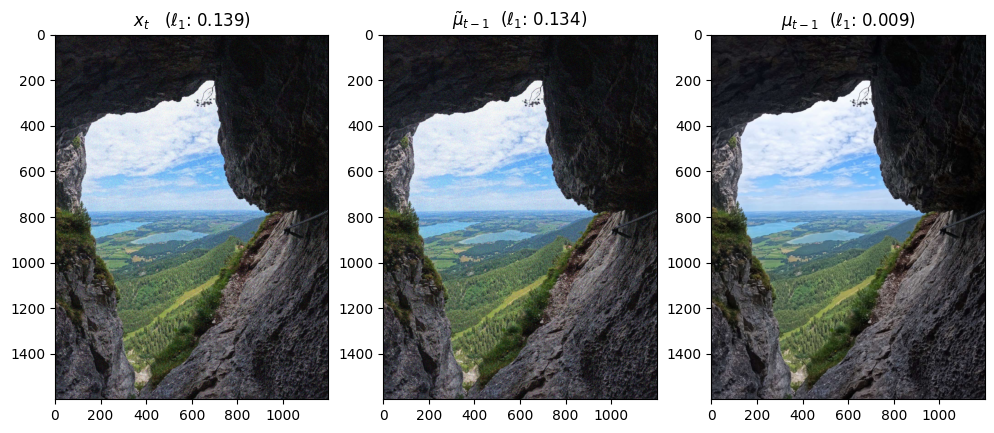
Approximation (or knowledge) of \(x_0\) allows us to approximate the mean of the step \(t-1\), using (4).
# estimate mean
mean_pred=x_0_pred*(alphas_cumprod_sqrt[t_step-1]*betas[t_step])/(1-alphas_cumprod[t_step]) + x_t*(alphas_sqrt[t_step]*(1-alphas_cumprod[t_step-1]))/(1-alphas_cumprod[t_step])

# let's compare it to ground truth mean of the previous step (requires knowledge of x_0)
mean_gt=alphas_cumprod_sqrt[t_step-1]*img_
Since reverse process mean estimation \(\tilde{\mu}_\theta\) in (4) is effectively linear interpolation between noisy \(x_t\) and \(x_0\) it is expected to have a higher error (as the additive noise is still present) compared to the mean computed using the forward process (which is computed by scaling the clean sample by a scalar value).
plt.subplot(1,3,1)
show(x_t)
plt.title('$x_t$   ($\ell_1$: {:.3f})'.format(F.l1_loss(x_t,img_)))
plt.subplot(1,3,2)
show(mean_pred)
plt.title(r'$\tilde{\mu}_{t-1}$' + '  ($\ell_1$: {:.3f})'.format(F.l1_loss(mean_pred,img_)))
plt.subplot(1,3,3)
show(mean_gt)
plt.title(r'$\mu_{t-1}$' + '  ($\ell_1$: {:.3f})'.format(F.l1_loss(mean_gt,img_)))
Text(0.5, 1.0, '$\\mu_{t-1}$ ($\\ell_1$: 0.009)')
Once we get our mean_pred (\(\tilde{\mu_{t}}\)), we can define our distribution for the previous step
Important: the experiment below should be treated as a simulation. In practice, the network must predict either \(\epsilon_\theta\) or \(x^{\theta}_0\) or \(\tilde{\mu}_\theta\). Here, the value of \(epsilon\) is simply subs
def reverse_step(epsilon, x_t, t_step, return_noise=False):

    # estimate x_0 based on epsilon
    x_0_pred=(x_t-(1-alphas_cumprod[t_step]).sqrt()*epsilon)/(alphas_cumprod_sqrt[t_step])
    if t_step==0:
        sample=x_0_pred
        noise=torch.zeros_like(x_0_pred)
    else:
        # estimate mean
        mean_pred=x_0_pred*(alphas_cumprod_sqrt[t_step-1]*betas[t_step])/(1-alphas_cumprod[t_step]) + x_t*(alphas_sqrt[t_step]*(1-alphas_cumprod[t_step-1]))/(1-alphas_cumprod[t_step])

        # compute variance
        beta_pred=betas[t_step].sqrt() if t_step != 0 else 0

        sample=mean_pred+beta_pred*torch.randn_like(x_t)
        # this noise is only computed for simulation purposes (since x_0_pred is not known normally)
        noise=(sample-x_0_pred*alphas_cumprod_sqrt[t_step-1])/(1-alphas_cumprod[t_step-1]).sqrt()
    if return_noise:
        return sample, noise
    else:
        return sample
x_t,noise=forward_jump(1000-1,img_,return_noise=True)

state_imgs=[x_t.numpy()]
for t_step in reversed(range(1000)):
    x_t,noise=reverse_step(noise,x_t,t_step,return_noise=True)

    if t_step % 200 == 0:
        state_imgs.append(x_t.numpy())
plt.figure()
for idx,state_img in enumerate(state_imgs):
    plt.subplot(1,len(state_imgs),idx+1)
    show(state_img.clip(-1,1))
    plt.axis('off')

plt.tight_layout()