
From Discrete Diffusion to Continous Time Diffusion Processes#
Remebmer the forward step of the diffusion process from the previous notebook: $\( q(\mathbf{x}_{1:T} \vert \mathbf{x}_0) = \prod^T_{t=1} q(\mathbf{x}_t \vert \mathbf{x}_{t-1}) , \quad q(x_t|x_{t−1}) := \mathcal{N}(x_t; \sqrt{1 − \beta_t}x_{t−1}, \beta_tI) \tag{1} \)$
We can rewrite the forward step using the reparameztrization trick as follows:
where \(\Delta t\) is the time step and we define \(\beta_t := \beta(t) \Delta t\).
Using smaller and smaller time steps \(\Delta t\) we can view the diffusion process using an infinite number of infinitely small time steps in the limit. Using Taylor expansion we can rewrite the forward step as follows: $\( x_t \approx x_{t−1} - \frac{\beta(t) \Delta t}{2} x_{t−1} + \sqrt{\beta(t) \Delta t} \mathcal{N}(0,\mathbf{I}) \tag{3} \)$
In the limit of \(\Delta t \rightarrow 0\) (continuous-time diffusion models) we obtain the following stochastic differential equation (SDE):
Here, \(x_t\) represents data, \(dx_t\) and \(dt\) are infinitesimal updates of data and time, \(dw_t\) is a noise process that corresponds to Gaussian noise injection, and \(\beta(t)\) is now a continuous function of time \(t\).
What are Stochastic Differential Equations (SDEs)?#
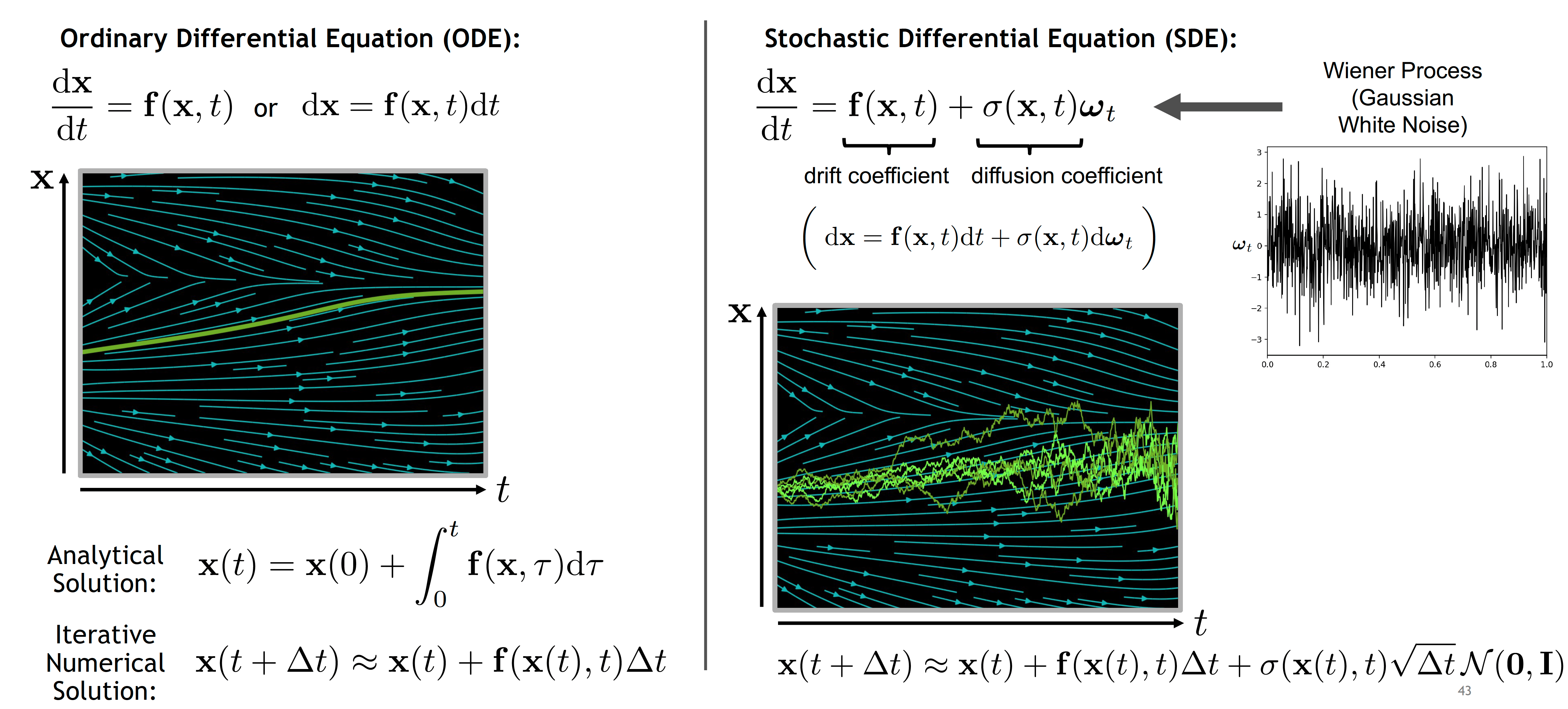
Stochastic Differential Equations (SDEs) are a type of differential equation in which one or more of the terms is a stochastic process, resulting in a solution that is also a stochastic process. They are used to model systems that are influenced by random effects. The Slide from the CVPR tutorial on Denoising Diffusion based Models (https://cvpr2022-tutorial-diffusion-models.github.io/) below helps to understand the difference between ODEs and SDEs:
To better understand SDEs, it’s important to first understand the concept of a stochastic process. A stochastic process is a mathematical object usually defined as a collection of random variables. For example for a collection of random variables with respect to time you can think of something like the likelihood of a position or motion of a particle over time. In the context of SDEs, these random variables represent the evolution of a system of random values over time.
As a solution for a Stochastic Differential Equation, the diffusion process is a type of stochastic process that is commonly used to model the dynamics of continuously changing phenomena where randomness plays a role. We can use it where we want to model some form of random walk or noise component. In a diffusion process, the change in the system over time is governed by two components:
Drift: This is the deterministic part of the process, which can be thought of as the “average” or “expected” direction in which the process moves. In an SDE, this is typically represented by a function of the current state and time.
Diffusion: This is the stochastic part of the process, which represents random fluctuations around the drift. In an SDE, this is typically represented by a function of the current state and time, multiplied by a Wiener process or another type of stochastic process.
The most common example of a diffusion process is Brownian motion, also known as the Wiener process, which models the random motion of particles suspended in a fluid. In Brownian motion, the drift is zero, so the motion is entirely random, with the current velocity of a particle independent of its past velocities. As an example of Brownian motion, the following animation shows a large particle, that collides with a large set of other smaller particles (like a dust particle in the air) and moves in a random directions:
In a more general diffusion process, the drift can be non-zero, so the process has a tendency to move in a certain direction, but there are still random fluctuations around this direction. For example with the SDE from above:
we have the following different parts of the general SDE of the form:
Where, \(x_t\) is the state of the system at time \(t\), \(a(x_t, t)=-\frac{1}{2}\beta(t)x_{t}\) is the deterministic part of the change in the system also referred to as the drift term, such as the average velocity of a particle in a fluid due to the fluid flow. The function \(b(x_t, t)=\sqrt{\beta(t)}\) is referred to as the diffusion coefficient, and the term \(\sqrt{\beta(t)} dw_{t}\) is the diffusion term. Here, \(dw_t\) represents an infinitesimal increment of a Wiener process (or Brownian motion), which is a continuous-time stochastic process with independent, normally distributed increments.
The diffusion term is responsible for the random fluctuations in the process \(x_t\). The function \(b(x_t, t)\) determines how these random fluctuations scale with the state of the system and time. For example, if \(b(x_t, t)\) is large, then the process \(x_t\) will have large random fluctuations, and vice versa. The diffusion term represents the random, unpredictable changes in the system, such as the random motion of particles in a fluid due to collisions with other particles. The drift term \(a(x_t,t)dt\) represents the average or expected change in the system, such as the average velocity of a particle in a fluid due to the fluid flow.
The deterministic part, \(a(x_t,t)dt\) is similar to what you would see in an ordinary differential equation (ODE). The stochastic part, \(b(x_t,t)dw_t\) is what differentiates an SDE from an ODE. This term introduces randomness into the system. The solution to an SDE is a stochastic process. This means that instead of a single curve as in an ODE, the solution to an SDE is a family of curves, or a random process. Each individual curve represents one possible “path” that the system could take, and the collection of all such curves gives a complete description of the system’s behavior.

How does this relate to the diffusion process for data generation?#
The deterministic drift part of the diffusion process pulls the data towards the mode of the data distribution. The stochastic diffusion part injects noise into the data. Because of the noise there is no unique path that the data takes. Instead, there is a family of curves that the data could take. The collection of all such curves gives a description of the data distribution. The image below helps to visualize this:
On the left we have samples of the data distribution (images of bedrooms). In the center we have the corresponding diffusion process. In red we can see actual sampled trajectories of the diffusion process. In blue to yellow we can see the a visualization of the probability density function over time. On the left side a simplified multimodal distribution like a Gaussian Mixture Model changing to a univariat Gaussian over time. We can see that there is a deterministic part which pulls the samples to the modes of the distribution and a stochastic part which injects noise making each trajectory unique. We can see that the diffusion process starts with the data distribution and ends with the unit Gaussian distribution.
How do we use this for data generation? - Reverse-time diffusion process#
If we can run this process in the reverse direction we could genereate data from the unit gaussian distribution. As shown in general by Brian Anderson in “Reverse-time diffusion equation models” (https://www.sciencedirect.com/science/article/pii/0304414982900515) and later by Yang Song for generative modeling in “Score-Based Generative Modeling through Stochastic Differential Equations” (https://arxiv.org/abs/2011.13456) we can run the diffusion process in reverse by solving the following SDE for the reverse time diffusion process:
Where, \(q_t(x_t)\) is the probability density function of the data distribution at time \(t\). The term \(-\beta(t)\nabla_{x_{t}}\log q_t(x_t)\) is the score function which is the gradient of the log probability of the data distribution. The score function forms the drift term together with the term \(-\frac{1}{2}\beta(t)x_{t}dt\), which is the same as in the forward direction. The diffusion term is also the same as in the forward diffusion SDE from above. We can use SDE solvers to generate data samples based on equation (7) (more on this later). However, there is the question how do we get the score function \(\nabla_{x_{t}}\log q_t(x_t)\)?