7.1 Predicting currents in the Openmanipulator joints with a neural network

7.1 Predicting currents in the Openmanipulator joints with a neural network#

In this part we will use a neural network to predict the currents in our Openmanipulator robot arm. We will use real measured data of the currents and the joint angles of the first joint of our robot to train a neural network. First we will import the data and plot it to get a better understanding of the data. Secondly we will preprocess the data and train a neural network. Finally we will evaluate the performance of our neural network.

import Pkg                                          # Package manager
# # Pkg.generate(joinpath(@__DIR__, "NeuronaleNetze"))  # activate package environment
Pkg.activate(joinpath(@__DIR__, "NeuronaleNetze"))  # activate package environment
Pkg.add("CSV")                                      # add CSV
Pkg.add("Plots")                                    # add Plots
Pkg.add("Statistics")                               # add Statistics
Pkg.add("ReverseDiff")                              # add ReverseDiff
Pkg.add("Flux")                                     # add Machine Learning Library Flux
Pkg.instantiate()

  Activating project at `~/Library/Mobile Documents/com~apple~CloudDocs/Projects/numerical_methods/07-NeuralNetworks/NeuronaleNetze`

    Updating registry at `~/.julia/registries/General.toml`

   Resolving package versions...

  No Changes to `~/Library/Mobile Documents/com~apple~CloudDocs/Projects/numerical_methods/07-NeuralNetworks/NeuronaleNetze/Project.toml`
  No Changes to `~/Library/Mobile Documents/com~apple~CloudDocs/Projects/numerical_methods/07-NeuralNetworks/NeuronaleNetze/Manifest.toml`

Precompiling project...

  ✓ GPUArrays

  ✓ Zygote

  ✓ Zygote → ZygoteColorsExt

  ✓ Flux

  ✓ NeuronaleNetze
  5 dependencies successfully precompiled in 40 seconds. 213 already precompiled.
   Resolving package versions...

  No Changes to `~/Library/Mobile Documents/com~apple~CloudDocs/Projects/numerical_methods/07-NeuralNetworks/NeuronaleNetze/Project.toml`
  No Changes to `~/Library/Mobile Documents/com~apple~CloudDocs/Projects/numerical_methods/07-NeuralNetworks/NeuronaleNetze/Manifest.toml`

Precompiling project...

  ✓ ColorVectorSpace → SpecialFunctionsExt

  ✓ ReverseDiff

  ✓ NeuronaleNetze
  3 dependencies successfully precompiled in 8 seconds. 215 already precompiled.
   Resolving package versions...

  No Changes to `~/Library/Mobile Documents/com~apple~CloudDocs/Projects/numerical_methods/07-NeuralNetworks/NeuronaleNetze/Project.toml`
  No Changes to `~/Library/Mobile Documents/com~apple~CloudDocs/Projects/numerical_methods/07-NeuralNetworks/NeuronaleNetze/Manifest.toml`

   Resolving package versions...

  No Changes to `~/Library/Mobile Documents/com~apple~CloudDocs/Projects/numerical_methods/07-NeuralNetworks/NeuronaleNetze/Project.toml`
  No Changes to `~/Library/Mobile Documents/com~apple~CloudDocs/Projects/numerical_methods/07-NeuralNetworks/NeuronaleNetze/Manifest.toml`

   Resolving package versions...

  No Changes to `~/Library/Mobile Documents/com~apple~CloudDocs/Projects/numerical_methods/07-NeuralNetworks/NeuronaleNetze/Project.toml`
  No Changes to `~/Library/Mobile Documents/com~apple~CloudDocs/Projects/numerical_methods/07-NeuralNetworks/NeuronaleNetze/Manifest.toml`

import Pkg                                          # Package manager
Pkg.activate(joinpath(@__DIR__, "NeuronaleNetze"))  # activate package environment
using CSV                                           # CSV Parser
using Plots                                         # Graph Plotter
using Statistics                                    # statisitical functions, like "mean"
using Flux                                          # Machine Learning Library
using ReverseDiff                                   # Reverse Mode Automatic Differentiation

  Activating project at `~/Library/Mobile Documents/com~apple~CloudDocs/Projects/numerical_methods/07-NeuralNetworks/NeuronaleNetze`

[ Info: Precompiling Flux [587475ba-b771-5e3f-ad9e-33799f191a9c]

[ Info: Precompiling SpecialFunctionsExt [997ecda8-951a-5f50-90ea-61382e97704b]

[ Info: Precompiling ZygoteColorsExt [e68c091a-8ea5-5ca7-be4f-380657d4ad79]

[ Info: Precompiling ReverseDiff [37e2e3b7-166d-5795-8a7a-e32c996b4267]

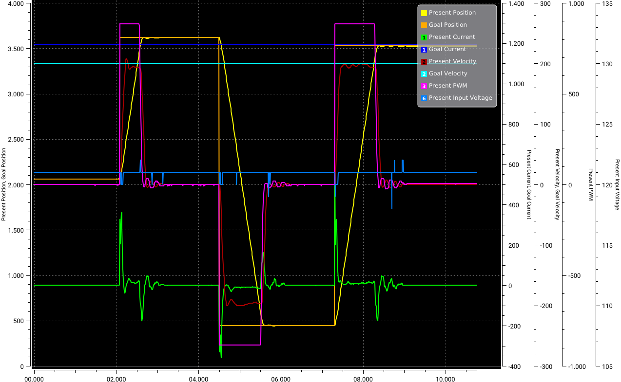
The Data#

Using the Openmanipulator we collected data using the Dynamixel Wizard tool which enables us to control and measure each actuator of our Robot. An image of the measured test data is shown below.

The data is stored in a CSV file. To load the CSV file, we can use the CSV module from Julia. For the input \(x\) into our model we will read the columns for:

Present Position
Goal Position
Present Velocity

We will make build the input matrix \(x\) of these values.

For the output \(y\) we will read the columns for:

Present Current

We will also make a matrix of these values. Since we are only predicting one value, we will only have one column. However, Flux expects a matrix, so we will make a matrix with one column.

function load_csv_data(filename)
    csv = CSV.File(filename)                        # load and parse csv
    x_1 = csv.columns[3].column                     # mask column 3 (Present Position) - input 1
    x_2 = csv.columns[4].column                     # mask column 4 (Goal Position) - input 2
    x_3 = csv.columns[7].column                     # mask column 7 (Present Velocity) - input 3
    y = csv.columns[5].column                       # mask column 5 (Present Current) - this is what we want to predict
    x_train = hcat(x_1, x_2, x_3)'                  # create input matrix
    y_train = y                                     # create output vector
    y_train = reshape(y_train, 1, :)                # reshape output vector to a matrix (1 x n) - this is what Flux expects
    x_train, y_train
end

load_csv_data (generic function with 1 method)

# load training data
x_train, y_train = load_csv_data(joinpath(@__DIR__, "OMP_Daten/pc-train.csv"))

# load test data
x_test, y_test = load_csv_data(joinpath(@__DIR__, "OMP_Daten/pc-test.csv"))

([2061 2061 … 3525 3525; 2061 2061 … 3526 3526; 0 0 … 0 0], [0 0 … 0 0])

To normalize the data we estimate the mean and standard deviation of the data.

mean_x = mean(x_train)
mean_y = mean(y_train)
std_x = std(x_train)
std_y = std(y_train)

74.32507644633692

Task: Functions for preprocessing and postprocessing the data#

If we want the distribution of our data x to have a mean of \(\mu = 0\) and a standard deviation of \(\sigma = 1\) we can use the following:

\[\begin{split} \mu_x = mean(x)\\ \sigma_x = std(x)\\ x_{norm} = (x - \mu_x)/\sigma_x \end{split}\]

Write a function to normalize the data using the mean and standard deviation.
Write a function to denormalize the data using the mean and standard deviation.

# data pre procseeing (make it machine frindly)
function dataPreProcess(x, y)
    x = Float32.(x)
    y = Float32.(y)
    x = (x .- mean_x) ./ std_x
    y = (y .- mean_y) ./ std_y
    x, y
end

# data post procseeing (make it human frindly)
function dataPostProcess(x, y)
    x = (x.* std_x) .+ mean_x
    y = (y.* std_y) .+ mean_y
    x, y
end

dataPostProcess (generic function with 1 method)

Preprocess the data using the function you wrote.

# Data Preprocessing
x_train, y_train = dataPreProcess(x_train, y_train)

([0.46310311404158183 0.46310311404158183 … 1.6074673134216337 1.6074673134216337; 0.46310311404158183 0.46310311404158183 … 1.6074673134216337 1.6074673134216337; -0.9706808124321389 -0.9706808124321389 … -0.9706808124321389 -0.9706808124321389], [-0.03509713558049676 -0.03509713558049676 … -0.04855154488368806 -0.03509713558049676])

Check the mean and std of the data to make sure we did it right.

@show mean(x_train)
@show std(x_train)
@show mean(y_train)
@show std(y_train);

mean(x_train) = 3.000783801098462e-17
std(x_train) = 1.0
mean(y_train) = 9.645376503530771e-18
std(y_train) = 1.0

We also need to normalize the test data. It is important to use the mean and std of the training data to normalize the test data since our neural network is trained on the normalized training data. Using a different mean and std for the test data would mean that we are using a different distribution for the test data than for the training data.

x_test, y_test = dataPreProcess(x_test, y_test)

([0.4736147264057587 0.4736147264057587 … 1.499548093149418 1.499548093149418; 0.4736147264057587 0.4736147264057587 … 1.50024886730703 1.50024886730703; -0.9706808124321389 -0.9706808124321389 … -0.9706808124321389 -0.9706808124321389], [-0.03509713558049676 -0.03509713558049676 … -0.03509713558049676 -0.03509713558049676])

Starting with a Linear Model#

In the lecture we showed that perceptrons can be build out of simple linear functions and adding a nonlinear activation layer. So before we will implement a neural network we take a step back and implement a linear function which estimates the currents.

The linear function is defined as:

\[ \tilde{y} = \tilde{x}^T \cdot \tilde{w} + b \]

where \(x\) is the input vector and \(w\) is the weight vector and \(b\) is the bias. We changed the notation to avoid adding the bias as a additional weight:

\[\begin{split} y = x^T \cdot w = \begin{bmatrix} 1 & x_1 & x_2 & \dots & x_n \end{bmatrix} \cdot \begin{bmatrix} w_b \\ w_1 \\ w_2 \\ \dots \\ w_n \end{bmatrix} = 1 \cdot w_b + x_1 \cdot w_1 + x_2 \cdot w_2 + \dots + x_n \cdot w_n \end{split}\]

where \(w\) is now the extended weight vector and \(x\) is the input vector extended by a 1.

First lets look at an example of how to calculate the output of the linear function. We will use the first 3 rows of the training data as an example. The weight vector \(w\) is used to generate an output \(y\) for each row of the matrix \(X\):

x_1 = x_train[:, 1:3] # first 3 training examples each having 3 values
@show x_1 = vcat(ones(1, size(x_1, 2)), x_1)
@show w_1 = [1, 1, 1, 1]
@show x_1' * w_1;

x_1 = vcat(ones(1, size(x_1, 2)), x_1) = [1.0 1.0 1.0; 0.46310311404158183 0.46310311404158183 0.46310311404158183; 0.46310311404158183 0.46310311404158183 0.46310311404158183; -0.9706808124321389 -0.9706808124321389 -0.9706808124321389]
w_1 = [1, 1, 1, 1] = [1, 1, 1, 1]
x_1' * w_1 = [0.9555254156510247, 0.9555254156510247, 0.9555254156510247]

Task: Build a linear model#

Build a linear model using the definition we gave above.

# forward propagation
function linear_forward(x, w)
    x = vcat(ones(1, size(x, 2)), x)

    # Calculate the output of the neuron
    y_hat = x' * w
end

# Define a function that takes in the weights and the data, and returns the loss
function loss(w, x, y)
    y_hat = linear_forward(x, w)
    mse = sum((y_hat .- y) .^ 2) / size(y, 1)
    return mse
end

# Define a function that computes the gradients of the loss with respect to the weights
function grad(w, x, y)
    return ReverseDiff.gradient(w -> loss(w, x, y), w)
end

# initialize model using random normal weights
function train_linear_model(x, y, learning_rate, num_epochs)
    w = randn(4, 1)
    mse = loss(w, x_t, y_t)
    println("Start: MSE = $mse")
    for i = 1:num_epochs
        # Compute the gradients of the loss with respect to the weights
        dw = grad(w, x, y)

        # Update the weights using gradient descent
        w -= learning_rate * dw

        if i % 10 == 0
            # Compute the loss and print it
            mse = loss(w, x, y)
            println("Iteration $i: MSE = $mse")
        end
    end
    return w
end

train_linear_model (generic function with 1 method)

Before we start to train a linear model on the real dataset we will generate an artificial one where we know that we can actually learn it using a linear function. We will use the following to generate the data:

using Random

# Set the random seed for reproducibility
Random.seed!(1234)

# Define the true weights
w_true = randn(3, 1)

# Generate the dataset
n_samples = 1000
x_t = randn(3, n_samples)
y_t = x_t' * w_true

# Add some noise to the targets
y_t += 0.1 * randn(n_samples, 1);

w = train_linear_model(x_t, y_t, 0.01, 200)

@show w_true
@show w;

Start: MSE = 0.9464013338542072

Iteration 10: MSE = 0.6410760962735835
Iteration 20: MSE = 0.4353207509809646
Iteration 30: MSE = 0.2966379543575615
Iteration 40: MSE = 0.20314550700729128
Iteration 50: MSE = 0.14010606536329417
Iteration 60: MSE = 0.09759230842309466
Iteration 70: MSE = 0.06891573177013914
Iteration 80: MSE = 0.04956910738880395
Iteration 90: MSE = 0.03651453827477731
Iteration 100: MSE = 0.02770407606575343
Iteration 110: MSE = 0.021756869759651243
Iteration 120: MSE = 0.01774169161162987
Iteration 130: MSE = 0.015030417226521634
Iteration 140: MSE = 0.013199290987990745
Iteration 150: MSE = 0.011962379619805737
Iteration 160: MSE = 0.01112671182101594
Iteration 170: MSE = 0.010562031244568221
Iteration 180: MSE = 0.010180398681443182
Iteration 190: MSE = 0.00992243374207581
Iteration 200: MSE = 0.009748033165807008
w_true = [-0.3597289068234817; 1.0872084924285859; -0.4195896169388487;;]
w = [0.009873818517424525; -0.35469544923317287; 1.104683290673515; -0.4143009593658289;;]

Task: Train the linear model on the current dataset#

Now lots try to train the model on the real data. We already extracted the data from the CSV file and normalized it. So we can just start the training process by passing x_trainand y_train to the train_linear_model function.

train_linear_model(x_train, y_train, 0.01, 200)

Start: MSE = 7.291819186390243

Iteration 10: MSE = 7.76168422366377e128

Iteration 20: MSE = 4.730999090933705e249

Iteration 30: MSE = Inf

Iteration 40: MSE = Inf

Iteration 50: MSE = Inf

Iteration 60: MSE = NaN

Iteration 70: MSE = NaN

Iteration 80: MSE = NaN

Iteration 90: MSE = NaN

Iteration 100: MSE = NaN

Iteration 110: MSE = NaN

Iteration 120: MSE = NaN

Iteration 130: MSE = NaN

Iteration 140: MSE = NaN

Iteration 150: MSE = NaN

Iteration 160: MSE = NaN

Iteration 170: MSE = NaN

Iteration 180: MSE = NaN

Iteration 190: MSE = NaN

Iteration 200: MSE = NaN

4×1 Matrix{Float64}:
 NaN
 NaN
 NaN
 NaN

Ok, this does not seem to work. Can you think of a reason why?

Task: Build a linear model using Flux#

We can also build and train a linear model in a few lines of code using FLux. Build a linear model using Flux and train it on the data.

using Flux
# building a linear  model using Flux
linear_model = Dense(3, 1)
                    

# Define the loss function
loss(x, y) = sum((linear_model(x) .- y) .^ 2) / size(y, 1)

# Define the optimizer
# opt = Descent(0.01) # you can also try it with the ADAM optimizer 
opt = ADAM(0.01)

# Train the model - check the train function and what we pass to it
# Note that the train function is called with train! which means that it will modify the model parameters passed to it
numIter = 200
for i in 1:numIter
    Flux.train!(loss, Flux.params(linear_model), [(x_train, y_train)], opt, cb=() -> println(loss(x_train, y_train)))
end

┌ Warning: Layer with Float32 parameters got Float64 input.
│   The input will be converted, but any earlier layers may be very slow.
│   layer = Dense(3 => 1)       # 4 parameters
│   summary(x) = "3×4420 Matrix{Float64}"
└ @ Flux ~/.julia/packages/Flux/pR3k3/src/layers/stateless.jl:60

913710690085
497538989885
4067578622
799507283413
8187978055
596126550869
244824441706
866801392363
545886113761
349424184522
328495612432
51726456128
9310670419
56687007451
405330024443
405959055548
512430545221
648237225319
719897243034
616823083517
209822552375
352913004886
885434867702
628476115785
389894077638
9623504808005
125607611502
647150626086
282234250188
776078369039
864328227399
273700755615
724104691919
929357604015
597433216772
432785217676
137474312449
411313353952
953516408124
4641765959805
644560302683
198683295788
83418144344
26321302579
202832106652
376722959518
515206217871
3561633768604
645764166348
1385843923167
5988964407247
800063580496
5256082474048
5691156623116
7343508667127
8356724930154
6979469179605
1562344233203
0560566135628
2531629647297
613408140926
0122373772338
334775864467
4752484493056
3367689906063
8309087321936
877336716091
403337995735
3435133872954
6392150330416
2381916775266
0941151314832
1661613790843
418583898764
8203178369804
34449815662
968183209594
671864988407
439177557274
256563875395
112942860472
999379749537
9088798298712
8360589904237
7769391284983
72872998986
6896741928554
6588304874585
635880293135
6210442861816
6149750674695
6185691829637
6329839653035
659465266551
699304215482
7538365727933
8243042284203
9119308398062
017768830686
142807744258
2878713091422
453635362819
640667802013
849293593003
079828514175
3323254960437
606799359529
9031016653717
2209924493195
5601322015914
920102701145
3004259190748
700516827941
1197637975165
557574998967
0132615510684
4861104526635
975465689017
4806159205214
0008602693033
535536932689
0839614309484
6454608289077
21944338715
8052784507
402424296002
0102919868955
6283593942862
2561520123013
8931704637525
5390184217376
1932255423185
855477247499
525351910371
2025282993327
8867099428567
5775800193524
2748624154074
9782942529628
6876450424834
4026824567536
123184602528
8489890040855
579837482975
315563191356
056076020969
8011036689377
5505444363234
3042514203134
0620574711693
823858344658
5894562994886
358791119743
131713739569
9081093618333
6878565021516
4708564289485
256973698428
04614688369
8382435215763
633184473755
430865423321
231190703256
0340904227037
8394595583586
647228007112
4573369656027
2696896816597
0842207736932
9008617556206
7195574035054
540225323823
3628185073285
187275168858
013535777336
841578046593
671292226722
50268391279
335705164678
170284571069
0064070646467
8440110589654
6830757713697
5235486923457
365403496533
2086419850475
053185494183
8990274371636
74612560319
5944686445896
4440229583183
29475215343
1466610736225
9997146124683
853881714872
709160005305
565504535969
42294156131
2813945398366
14087922401

Linear model with nonlinear activation function using Flux#

Now we extend the linear model by adding a nonlinear activation function. We will use the sigmoid function as activation function using Flux.sigmoid. Our function is then defined as:

\[\begin{split} y = h(x^T \cdot w) = h(\begin{bmatrix} 1 & x_1 & x_2 & \dots & x_n \end{bmatrix} \cdot \begin{bmatrix} w_b \\ w_1 \\ w_2 \\ \dots \\ w_n \end{bmatrix}) = h(1 \cdot w_b + x_1 \cdot w_1 + x_2 \cdot w_2 + \dots + x_n \cdot w_n) \end{split}\]

where \(h\) is the sigmoid function.

# build linear model with nonlinear sigmoid activation function
non_linear_model = Dense(3, 1, Flux.tanh)

# Define the loss function
loss(x, y) = sum((non_linear_model(x) .- y) .^ 2) / size(y, 1)

# Define the optimizer
opt = Descent(0.01) # you can also try it with the ADAM optimizer 

# Train the model
numIter = 200
for i in 1:numIter
    Flux.train!(loss, Flux.params(non_linear_model), [(x_train, y_train)], opt, cb=() -> println(loss(x_train, y_train)))
end

000000000004
000000000004
000000000004
000000000004
000000000004
000000000004
000000000004
000000000004
000000000004
000000000004
000000000004
000000000004
000000000004
000000000004
000000000004
000000000004
000000000004
000000000004
000000000004
000000000004
000000000004
000000000004
000000000004
000000000004
000000000004
000000000004
000000000004
000000000004
000000000004
000000000004
000000000004
000000000004
000000000004
000000000004
000000000004
000000000004
000000000004
000000000004
000000000004
000000000004
000000000004
000000000004
000000000004
000000000004
000000000004
000000000004
000000000004
000000000004
000000000004
000000000004
000000000004
000000000004
000000000004
000000000004
000000000004
000000000004
000000000004
000000000004
000000000004
000000000004
000000000004
000000000004
000000000004
000000000004
000000000004
000000000004
000000000004
000000000004
000000000004
000000000004
000000000004
000000000004
000000000004
000000000004
000000000004
000000000004
000000000004
000000000004
000000000004
000000000004
000000000004
000000000004
000000000004
000000000004
000000000004
000000000004
000000000004
000000000004
000000000004
000000000004
000000000004
000000000004
000000000004
000000000004
000000000004
000000000004
000000000004
000000000004
000000000004
000000000004
000000000004
000000000004
000000000004
000000000004
000000000004
000000000004
000000000004
000000000004
000000000004
000000000004
000000000004
000000000004
000000000004
000000000004
000000000004
000000000004
000000000004
000000000004
000000000004
000000000004
000000000004
000000000004
000000000004
000000000004
000000000004
000000000004
000000000004
000000000004
000000000004
000000000004
000000000004
000000000004
000000000004
000000000004
000000000004
000000000004
000000000004
000000000004
000000000004
000000000004
000000000004
000000000004
000000000004
000000000004
000000000004
000000000004
000000000004
000000000004
000000000004
000000000004
000000000004
000000000004
000000000004
000000000004
000000000004
000000000004
000000000004
000000000004
000000000004
000000000004
000000000004
000000000004
000000000004
000000000004
000000000004
000000000004
000000000004
000000000004
000000000004
000000000004
000000000004
000000000004
000000000004
000000000004
000000000004
000000000004
000000000004
000000000004
000000000004
000000000004
000000000004
000000000004
000000000004
000000000004
000000000004
000000000004
000000000004
000000000004
000000000004
000000000004
000000000004
000000000004
000000000004
000000000004
000000000004
000000000004
000000000004
000000000004
000000000004
000000000004

Neural Network#

Now we have seen that we cannot learn the current of the actuators using a linear model. We also adapted the linear model with a nonlinear activation function. Now we will use several layers of these linear functions with nonlinear activation function to build a feed forward neural network. We will use a fully connected feed forward neural network with 1-2 hidden layers and a linear output layer. To build such a fully connected feed forward neural network we can use the chain function from Flux. The chain function takes a list of layers as input and builds a neural network with these layers. In this case we will use Dense layers which are fully connected layers. The Dense layer takes the number of input neurons, the number of output neurons and the activation function as input.

Task: Build the neural network#

Build a neural network with 1-2 hidden layer. The input layer should have 3 neurons and the output layer should have 1 neuron to fit our data. You can also test different activation functions and different numbers of neurons in the hidden layer.

You can check the different activation function in flux here: https://fluxml.ai/Flux.jl/stable/models/activation/

To optimize the neural network we will use the ADAM optimizer and set its learning rate to \(0.001\). You can check the different optimizers in flux here: https://fluxml.ai/Flux.jl/stable/training/optimisers/

# define our Neural Network model
function build_model()
    opt = ADAM(0.001)
    input_size = size(x_train)[1]
    output_size = size(y_train)[1]
    model = Chain(Dense(input_size, 32, relu),
        Dense(32, 32, relu),
        Dense(32, output_size, identity))
    model, opt
end

build_model (generic function with 1 method)

Task: define the forward function#

We also define a forward function to calculate the output of the neural network.

function forward(x)
    y_hat = model(x)
end

forward (generic function with 1 method)

Task: define the loss function#

We also need a loss function to optimize. Since we are doing regression, we will use the mean squared error loss function. You can check the different loss functions in flux here: https://fluxml.ai/Flux.jl/stable/models/losses/

# Mean square error as the loss function for optimization
function loss(y_hat, y)
    sum((y_hat .- y) .^ 2)
end

loss (generic function with 2 methods)

Task: Train the neural network#

Now we will put everything together and train the neural network. We will define a function which takes the neural network, the optimizer, and the number of epochs as input. The function should return the loss based on the training and test data.

# train the model
function train_model(model, opt, numIter)
    trainLoss = zeros(numIter)
    testLoss = zeros(numIter)
    opt_state = Flux.setup(opt, model)
    for i in 1:numIter
        Flux.train!(model, [(x_train, y_train)], opt_state) do m, x, y
            loss(m(x), y)
        end
        trainLoss[i] = loss(forward(x_train), y_train) / length(y_train)
        testLoss[i] = loss(forward(x_test), y_test) / length(y_test)
    end
    trainLoss, testLoss
end

train_model (generic function with 1 method)

Calling the build_model() and train_model() functions:

model, opt = build_model() # build model
trainLoss, testLoss = train_model(model, opt, 1000) # train model

([1.0404954178824837, 1.0285629720485543, 1.017815951617186, 1.0082485489397477, 0.9997252074294303, 0.9920813242593242, 0.9851829202102648, 0.9788624355497945, 0.972989111670157, 0.9674405189160014  …  0.2174361180080419, 0.217370944007769, 0.21728451948155164, 0.2171750755469239, 0.21704500367468335, 0.2169052891127391, 0.21676045550053588, 0.216631430784194, 0.2165241132571936, 0.21644143808898125], [0.48593526444818375, 0.4748848904272836, 0.4652117723717658, 0.457062131596801, 0.4502811758449016, 0.4445673953083006, 0.43978542397853015, 0.435733750980032, 0.43217385460098906, 0.4288505615250615  …  0.08996966574812512, 0.09186244920673922, 0.08975519515549303, 0.0916835265351677, 0.08970905910395766, 0.0912221726020237, 0.08991361642104072, 0.09048910576676693, 0.09035815498838777, 0.08987093449581995])

Plotting the train and test loss:

# plot the train loss 
plot(trainLoss, label="Train Loss", xlabel="Iterations", ylabel="loss")

# plot the test loss
plot!(testLoss, label="Test Loss", xlabel="Iterations", ylabel="loss")

Let’s also plot the predicted currents and the actual currents based on the training data:

# plot the results for the training data
y_hat = forward(x_train)
plot(y_train[1, :], label="Ground Truth (train)", ylabel="Current")
plot!(y_hat[1, :], label="Prediction (train)")

Let’s do the same for the test data:

# test the final model on the test data
y_hat = forward(x_test)
error = sum((y_hat .- y_test) .^ 2) / length(y_test)
println("Test Error: ", error)

# post process the data (make it human readable)
x_test, y_test = dataPostProcess(x_test, y_test)
_, y_hat = dataPostProcess(x_test, y_hat)

# plot the results
plot(y_test[1, :], label="Ground Truth (test)", ylabel="Current")
plot!(y_hat[1, :], label="Prediction (test)")

# error in human readable form
error = y_hat .- y_test

# plot the error
plot!(error[1, :], label="Error", ylabel="Error")

Test Error: 0.08987093449581995

Could we replace a simulation with a neural network?#

In this part we will investigate how well a neural network can predict the change of the joint angle of the first joint of the Openmanipulator-X based on the joint angle, the goal joint angle and the current in the actuator.

function load_csv_data(filename)
    csv = CSV.File(filename)                        # load and parse csv
    x_1 = csv.columns[3].column[1:end-1]            # mask column 3 (Present Position) 
    x_2 = csv.columns[4].column[1:end-1]            # mask column 4 (Goal Position) 
    x_3 = csv.columns[5].column[1:end-1]            # mask column 5 (Present Current) 
    # the prediction will be the delta position of the joint (Present Position at time t+1 - Present Position at time t)
    y = csv.columns[3].column[2:end] - csv.columns[3].column[1:end-1] # mask column 3 (delta Position) - this is what we want to predict

    x_train = hcat(x_1, x_2, x_3)'                  # create input matrix
    y_train = y                                     # create output vector
    y_train = reshape(y_train, 1, :)                # reshape output vector to a matrix (1 x n) - this is what Flux expects
    x_train, y_train
end

load_csv_data (generic function with 1 method)

# load training data
x_train, y_train = load_csv_data(joinpath(@__DIR__, "OMP_Daten/pc-train.csv"))
# load test data
x_test, y_test = load_csv_data(joinpath(@__DIR__, "OMP_Daten/pc-test.csv"))

([2061 2061 … 3525 3525; 2061 2061 … 3526 3526; 0 0 … 0 0], [0 0 … 0 0])

Lets plot the training data to get a better understanding of the data:

# plot the data and set the heading 
p1 = plot(x_train[1, :], label="P-Pos", ylabel="x_1")
p2 = plot(x_train[2, :], label="G-Pos", ylabel="x_2")
p3 = plot(x_train[3, :], label="P-I", ylabel="x_3")
p4 = plot(y_train[1, :], label="∂-Pos", ylabel="y")

plot(p1, p2, p3, p4, layout=(4, 1))

Normalize the data:

# calculate mean and standard deviation of the training data
mean_x = mean(x_train)
mean_y = mean(y_train)
std_x = std(x_train)
std_y = std(y_train)
# Data Preprocessing
x_train, y_train = dataPreProcess(x_train, y_train)
x_test, y_test = dataPreProcess(x_test, y_test)

([0.4741199295295133 0.4741199295295133 … 1.5008998289755333 1.5008998289755333; 0.4741199295295133 0.4741199295295133 … 1.5016011813658654 1.5016011813658654; -0.9713673469446992 -0.9713673469446992 … -0.9713673469446992 -0.9713673469446992], [-0.02003504923446377 -0.02003504923446377 … -0.02003504923446377 -0.02003504923446377])

Now we build the model and train it. This time we will train it for \(20000\) epochs. The rest of the parameters stay the same.

model, opt = build_model() # build model
trainLoss, testLoss = train_model(model, opt, 20000) # train model

([1.0228227214352001, 0.9965736005250969, 0.9713614819069315, 0.9472253978897653, 0.9241210379544437, 0.9019925339522422, 0.8807524413520813, 0.8603005902150264, 0.840594735329256, 0.8215905536316962  …  0.004471555799321393, 0.004474152789156546, 0.004476836473598991, 0.004480359682074878, 0.0044837654904354715, 0.004488161261447957, 0.00449241915864023, 0.00449713085261265, 0.004501766470505711, 0.004508047973317812], [0.6864295240501983, 0.6645025907139858, 0.6438979845255944, 0.6246338660548105, 0.6066765100605235, 0.5899084748280882, 0.5742130991294334, 0.5594753129784247, 0.545688795919504, 0.5327951963422685  …  0.002043555236727043, 0.0020900571115619925, 0.002050709934658085, 0.002102025327968878, 0.0020542891208735403, 0.0021171765520147665, 0.0020624494016207727, 0.00213532530581838, 0.002070472361886978, 0.002153709882977916])

Let’s plot the train and test loss:

# plot the train loss
fig = plot(1:numIter, trainLoss, label="Train Loss", xlabel="Iterations", ylabel="loss")
# plot the test loss
plot!(1:numIter, testLoss, label="Test Loss", xlabel="Iterations", ylabel="loss")

Check how well the model predicts the joint angle change based on the training data:

# plot the results for the training data
y_hat = forward(x_train)
plot(y_train[1, :], label="Ground Truth (train)", ylabel="Position")
plot!(y_hat[1, :], label="Prediction (train)")