6.1 Linear Least Squares Tasks

6.1 Linear Least Squares Tasks#

Simple Setup to get started#

First, we’ll need to generate a set of data points that roughly follow a linear trend but with some noise added. We’ll use the function \(f(x) = 2x + 3\) to generate the \(y_i\) values. We’ll then add some Gaussian noise to the \(y_i\) values to simulate real-world measurements.

using Pkg
# Pkg.generate("learningF")
Pkg.activate("learningF")
Pkg.add("Plots")
Pkg.add("Statistics")
Pkg.add("CSV")
Pkg.instantiate()

  Activating project at `~/Library/Mobile Documents/com~apple~CloudDocs/Projects/numerical_methods/06-LeastSquares/learningF`

   Resolving package versions...

  No Changes to `~/Library/Mobile Documents/com~apple~CloudDocs/Projects/numerical_methods/06-LeastSquares/learningF/Project.toml`
  No Changes to `~/Library/Mobile Documents/com~apple~CloudDocs/Projects/numerical_methods/06-LeastSquares/learningF/Manifest.toml`

   Resolving package versions...

  No Changes to `~/Library/Mobile Documents/com~apple~CloudDocs/Projects/numerical_methods/06-LeastSquares/learningF/Project.toml`
  No Changes to `~/Library/Mobile Documents/com~apple~CloudDocs/Projects/numerical_methods/06-LeastSquares/learningF/Manifest.toml`

   Resolving package versions...

  No Changes to `~/Library/Mobile Documents/com~apple~CloudDocs/Projects/numerical_methods/06-LeastSquares/learningF/Project.toml`
  No Changes to `~/Library/Mobile Documents/com~apple~CloudDocs/Projects/numerical_methods/06-LeastSquares/learningF/Manifest.toml`

using Plots
using Statistics
using CSV                               # CSV Parser

# Generate x values
x = LinRange(-10, 10, 100)

# Generate y values with added noise
y = 2 .* x .+ 3 + randn(length(x))

# Plot the data points
scatter(x, y, label="Data Points")

Task: Matrix Formation#

The next step is to form the matrix \(A\).

Construct the matrix \(A\). Remember, the first column should be all ones (for the constant term in the linear function) and the second column should be the \(x_i\) values.

n = length(x)
A = [ones(n) x]

100×2 Matrix{Float64}:
0  -10.0
0   -9.79798
0   -9.59596
0   -9.39394
0   -9.19192
0   -8.9899
0   -8.78788
0   -8.58586
0   -8.38384
0   -8.18182
0   -7.9798
0   -7.77778
0   -7.57576
 ⋮    
0    7.77778
0    7.9798
0    8.18182
0    8.38384
0    8.58586
0    8.78788
0    8.9899
0    9.19192
0    9.39394
0    9.59596
0    9.79798
0   10.0

Task: Solving the Normal Equations#

Now, we are ready to solve the normal equations to get the least squares solution.

Compute the matrix \(A^T A\) and the vector \(A^T y\) in a seperate cell and view the results.

# Compute the matrix $A^T A$ and the vector $A^T y$
AtA = A' * A

2×2 Matrix{Float64}:
 100.0             6.39488e-14
   6.39488e-14  3400.67

# Compute the vector $A^T y$
Aty = A' * y

2-element Vector{Float64}:
  311.31154981759823
 6879.981679478033

Solve the system of equations \(A^T A p = A^T y\) to find \(p\)

# Solve the linear system $A^T A p = A^T y$
p = AtA \ Aty

2-element Vector{Float64}:
 3.113115498175981
 2.023123325549481

Task: Verification#

Finally, verify the solution you obtained.

Compute the residuals \(r_i\) and the total mean squared error.
Plot the original data points, the true line \(f(x)\), and the line corresponding to your solution.

# Compute the residuals $r_i$ and the total mean squared error
residuals = y - A * p
error = Statistics.mean(residuals .^ 2)

0.936794490723092

# Plot the original data points, the true line $f(x)$, and the line corresponding to your solution.
plot!(x, p[1] .+ p[2] .* x, label="Least Squares Solution")
plot!(x, 2 .* x .+ 3, label="True Line")

Task: Using the Julia built-in function#

You can use also the build in function \ to solve linear equations in Julia since it uses the least squares method if the system is overdetermined.

Build a linear equation of type \(Ax=b\) and solve it with the \ function. Compare the result with the solution you obtained erlier.

# Solve the linear equation using the build in function
A = [ones(length(x)) x]
b = y
p = A \ b

# Compute the residuals $r_i$ and the total mean squared error
residuals = y - A * p
error = Statistics.mean(residuals .^ 2)
println("Error: ", error)

# Plot the original data points, the true line $f(x)$, and the line corresponding to your solution.
plot!(x, p[1] .+ p[2] .* x, label="Least Squares Solution")
plot!(x, 2 .* x .+ 3, label="True Line")

Error: 0.9367944907230918

Task: Implement a function that computes the least squares solution#

Now we want to implement a function that computes the least squares solution for a given set of data points \((x_i, y_i)\), \(i=1,\ldots,n\).

Implement a function least_squares that takes as input the vectors \(x\) and \(y\) and returns the least squares solution \(p^*\) together with the matrix \(A\).

function least_squares(x, y)
    n = length(x)
    A = [ones(n) x]
    b = y
    p = A \ b
    p, A
end

least_squares (generic function with 1 method)

p, A = least_squares(x, y)
residuals = y - A * p
error = Statistics.mean(residuals .^ 2)
println("Error: ", error)

Error: 0.9367944907230918

Linear Least Squares using real world data#

We measured the current \(I\) of the first joint of our Openmanipulator robot for different goal currents \(I_g\) and obtained the following data points seen in the image below:

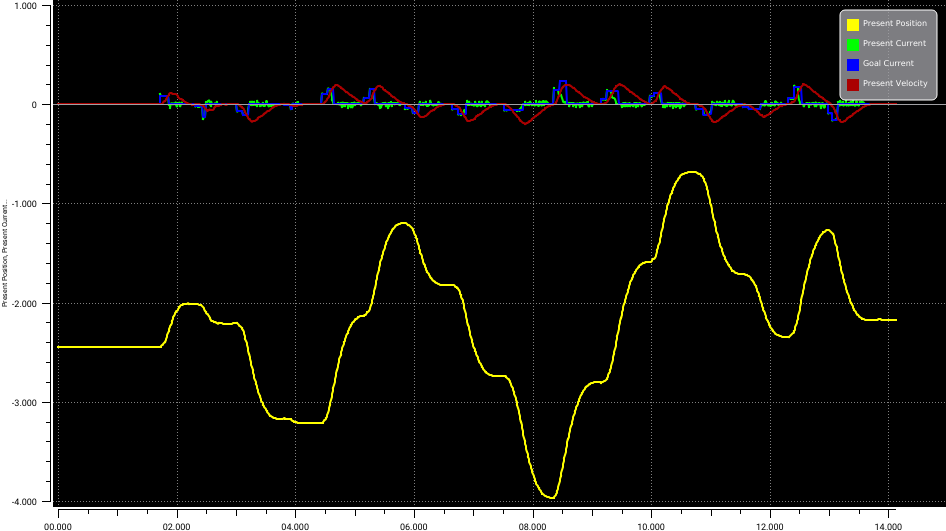
We want to find a linear function \(I = f(I_g)\) that describes the relationship between the goal current \(I_g\) and the actual current \(I\). We want to know how accuarate we can predict the actual current \(I\) for a given goal current \(I_g\). Fist let’s load the data points into Julia.

csv = CSV.File(joinpath(@__DIR__, "omp_currents.csv"))      # load and parse csv

x_train = csv.columns[5].column                      # mask column 5 (Goal Current)
y_train = csv.columns[4].column                      # mask column 4 (Present Current)

# x_train = x[1:1000]                       # take the first 800 values
# y_train = y[1:1000]                       # take the first 800 values

mean = Statistics.mean(x_train)           # calculate the mean
std = Statistics.std(x_train)             # calculate the variance

function dataPreProcess(x, y)
    x = Float64.(x)
    y = Float64.(y)
    # make the data zero mean and unit variance
    x = x .- mean
    x = x ./ std
    y = y .- mean
    y = y ./ std
    x, y
end

# data post procseeing (make it human frindly)
function dataPostProcess(x, y)
    x = x .* std
    x = x .+ mean
    y = y .* std
    y = y .+ mean
    x, y
end

# data pre processing
x_train, y_train = dataPreProcess(x_train, y_train)

([1.4967109895580646, 1.4967109895580646, 1.4967109895580646, 1.4967109895580646, 1.4967109895580646, 1.4967109895580646, 1.4967109895580646, 1.4967109895580646, 1.4967109895580646, 1.4967109895580646  …  -0.06866143611634576, -0.06866143611634576, -0.06866143611634576, -0.06866143611634576, -0.06866143611634576, -0.06866143611634576, -0.06866143611634576, -0.06866143611634576, -0.06866143611634576, -0.06866143611634576], [1.7486100005861305, 1.460725416554055, 1.4967109895580646, 1.4967109895580646, 1.4787182030560597, 1.4787182030560597, 1.4787182030560597, 1.4787182030560597, 1.4427326300520504, 1.4787182030560597  …  -0.06866143611634576, -0.06866143611634576, -0.06866143611634576, -0.06866143611634576, -0.06866143611634576, -0.06866143611634576, -0.06866143611634576, -0.06866143611634576, -0.06866143611634576, -0.06866143611634576])

# plot the goal current vs the present current
plot(x_train, label="Goal Current")
plot!(y_train, label="Present Current")

Task: Compute the parameters of the linear function#

Now we want to compute the parameters \(p_1\) and \(p_2\) of the linear function \(I = f(I_g) = p_1*I_g + p_2\) that best fits the data points.

Compute the parameters \(a\) and \(b\) of the linear function \(I = f(I_g) =p_1*I_g + p_2\) that best fits the data points using the least squares method you implemented earlier.
Estimate the mean squared error of the linear function.

p, A = least_squares(x_train, y_train)
residuals = y_train - A * p
error = Statistics.mean(residuals .^ 2)
println("Error: ", error)

Error: 0.1878335628013888

# Plot the original data points and the line corresponding to your solution
scatter(x_train, y_train, xlabel="Goal Current", ylabel="Present Current", label="Training Data", legend=:topleft)
# plot the least squares solution
plot!(x_train, p[1] .+ p[2] .* x_train, label="Least Squares Solution")

Solving underdetermined systems using the pseudoinverse#

If we have a linear system \(Ax = b\) with more unknowns than equations, i.e. \(A\) is rank deficient, then we cannot use the known tools to find a solution \(x\) such that \(Ax = b\). We can however define:

\[ B = A^T \]

and use the pseudoinverse of \(B^+\)

\[ B^+ = (B^T B)^{-1} B^T \]

with

\[ (B^+)^T = A^T (A A^T)^{-1} \]

Hence, if we use the pseudoinverse of the system we find the solution with minimal norm, i.e. the solution that minimizes \(\|x\|\). In this exercise we will use the pseudoinverse to find the least squares solution of an underdetermined system of equations.

Setup#

We first need to create an underdetermined system of equations. Let’s make this system a little simpler for ease of computation.

# A 2x3 matrix $A$ with random values.
A = rand(2, 3)

# 2-dimensional vector $b$ also with random values.
b = rand(2)

2-element Vector{Float64}:
 0.25754293001244
 0.708171825031344

Task: Compute the Pseudoinverse#

Now we will compute the pseudoinverse \(B^+\) of the transposed matrix \(B = A^T\).

Compute the matrix \(B\) by transposing \(A\).
Compute the pseudoinverse \(B^+\) using the formula provided. Note that this might involve computing a matrix inverse.

# Compute the matrix $B$ by transposing $A$.
B = A'

# Compute the pseudoinverse $B^+$ using B^+ = (B^T B)^{-1} B^T
B⁺ = inv(B' * B) * B'

2×3 Matrix{Float64}:
  1.76385   0.501003  -0.668612
 -0.632484  0.126246   1.37749

Task: Solve the Underdetermined System#

With the pseudoinverse \(B^+\), we can now solve for \(x\).

Compute the solution \(x = (B^+)^T b\).
Print the solution \(x\).

# Compute the solution $x = (B^+ b$.
x = B⁺' * b

# Print the solution $x$.
println("x = ", x)

x = [0.006360661435481018, 0.21843389190123785, 0.8033033290296383]

Task: Verification#

Finally, we should verify the solution we obtained.

Compute the vector \(Ax\) and compare it with \(b\). Given that we have an underdetermined system, they do not have to be the same.
Compute the norm of \(x\)
Compare your solution with the one obtained using the function \. Also compare the norm of the solution obtained with \ with the norm of the solution obtained with the pseudoinverse.

# Compute the vector $Ax$ and compare it with $b$. Given that we have an underdetermined system, they are not likely to be the same.
println("Ax = ", A * x)
println("b = ", b)

# Compute the norm of $x$ and discuss why this solution is preferable when we have an underdetermined system.
println("norm(x) = ", Statistics.norm(x))

# compare to \
x = A \ b
println("x = ", x)
println("norm(x) = ", Statistics.norm(x))

Ax = [0.25754293001244, 0.708171825031344]
b = [0.25754293001244, 0.708171825031344]
norm(x) = 0.832496283220002
x = [0.0063606614354812675, 0.21843389190123794, 0.8033033290296383]
norm(x) = 0.832496283220002

6.1 Linear Least Squares Tasks

Contents

6.1 Linear Least Squares Tasks#

Simple Setup to get started#

Task: Matrix Formation#

Task: Solving the Normal Equations#

Task: Verification#

Task: Using the Julia built-in function#

Task: Implement a function that computes the least squares solution#

Linear Least Squares using real world data#

Task: Compute the parameters of the linear function#

Solving underdetermined systems using the pseudoinverse#

Setup#

Task: Compute the Pseudoinverse#

Task: Solve the Underdetermined System#

Task: Verification#